Sign In

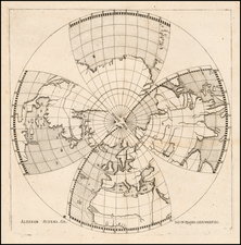
The Earliest Global Coverage of Isogonic Lines -- "a very useful light for navigation and physics"

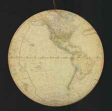
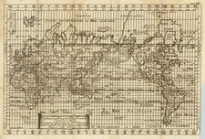
Rare pair of maps showing the northern and southern hemispheres on a polar projection and illustrating magnetic variation with isogonic lines, based upon the observations of Nicolaas Van Ewyk, a captain in the Dutch East India Company (VOC) in 1750. 

This is almost certainly the earliest example of isogonic lines covering the entire globe, as well as the first to cover the poles. It improves on the work of other savants like Halley and Van Musschenbroeck. 

The hemispheres mark longitude in their outer circle. There is another circle just inside this one with numbers from one to twenty, ascending and descending as one travels east to west. These are measurements of magnetic variation; the lines radiating from them are isogonic lines, showing places where that variation is equal.

A double line runs through the chart; it splits the variation readings between northwest and northeast, like a geomagnetic prime meridian. On both hemispheres, the magnetic pole is marked. In the north, a letter “N” marks the spot, in Hudson’s Bay. In the south, the pole is marked with a letter “Z” and is located just inside the eastern edge of the Antarctic Circle. These conventions are explained in French and Dutch in the lower corners.

The maps were by Nicolas van Ewyk, a captain in the VOC who hoped these maps would be a “very useful light for navigation and physics,” as he states in the maps’ titles. Van Ewyk commanded voyages to the East Indies, making navigational observations as he sailed.

The geography of the maps is also of interest. There is no southern continent and Van Diemen’s Land (Tasmania) and New Zealand are just unfinished coast lines, awaiting further exploration. The Australian coastline nearly connects to New Guinea; it is peppered with toponyms based on Dutch interactions over the course of the seventeenth century.

The southern hemisphere is covered in isogonic lines, but it is also ringed in several ships’ tracks. These include the 1738-9 voyage of Bouvet de Lozier. On this voyage in the South Atlantic and Indian Oceans Bouvet de Lozier sighted land, which he called Cap de la Circoncision, and reported massive icebergs at sea.

Also here is Edmond Halley’s track. Halley convinced the British Admiralty to give him a ship, the Paramore, to use as a mobile laboratory for studying magnetic variation on three voyages at the turn of the eighteenth century. On his second voyage, Halley took the Paramore into the Southern Atlantic, as seen here. While there, he nearly lost his ship to the soaring icebergs he encountered.

Nearby is the route of William Dampier in 1700. Dampier was the first person to circumnavigate the world three times. In doing so, he named the island of New Britain, off New Guinea, which is seen here. In Australia, he gave the name Sharks Bay (here Scharks bay). He also provided one of the earliest printed descriptions of Aboriginal peoples in Europe. Unfortunately, it was not a positive description, shaping harmful stereotypes for centuries to come.

In the Pacific are the lines of the voyages of Mendaña (1568 and 1595) and Ferdinand de Quiros in search of the Solomon Islands and the great southern continent in the late sixteenth and early seventeenth centuries. On his 1605 voyage, Quiros encountered what he called Austrialia de Espiritu Santo, which is actually Vanuatu. The exaggerated landmass is marked prominently on this map.

Magellan’s historic inaugural circumnavigation route, which passes through the Straits of Magellan, departs westward from the Straits. The voyage of Schouten and Le Maire is also marked, a circumnavigation in 1615-6 that found an alternative route to the Pacific, bypassing the Straits of the Magellan. The Dutchmen went instead around Cape Horn.

Crossing between the hemispheres is the trans-Pacific route of Anson. Commodore George Anson completed a circumnavigation as part of a bellicose voyage to harass Spanish trade in the Pacific from 1740 to 1744. Although he lost 1,500 of his 1,900 men and five of his six ships, Anson managed to capture the Acapulco treasure galleon off the coast of the Philippines.

Anson’s track is the only one in the northern hemisphere. Although there are unfinished coastlines near the North Pole, the difficulty of passing from Atlantic to Pacific in the icy waters is clear. However, there are possible passages suggested, via Baffin’s Bay or around Greenland. The extent of Terre de la Compagnie in the North Pacific is also left unsettled.

The History of Geomagnetism

The maps show an interim stage in the measurement and illustration of geomagnetism. Humans have known for centuries that there was a magnetic property to metals, and to navigation. Polarity and orientation were first recorded in China in the sixth century; they also recorded the first compasses, a needle floating in a bowl of water, in the twelfth century. This technique for finding direction was also developed in Europe in the Medieval period. The first maps to include an inkling of declination are markings on German sundials from the mid-fifteenth century. Soon mapmakers adopted the convention, including declination markings on their wind roses.

Until the sixteenth century, the seat of magnetic attraction was thought to be housed in the heavens. In the early modern period, more and more data was gathered. This data was collected by navigators at sea and consisted of magnetic inclination, declination, and deviation. The former, also known as magnetic dip or the dip angle, is the angle made with the horizontal by the Earth’s magnetic fields. Magnetic declination, or variation, is the angle on a horizontal plane between magnetic and true north. Magnetic deviation is the affect of local magnetic fields on compass error. Directional data led savants to conclude that these phenomena varied considerably based on one’s location. They found there was terrestrial polar attraction, creating waves, or lines, of magnetic variation across the globe.

More data also shifted understanding of the source of magnetic variety. As more and more ships took to the open seas, they contributed new data sets. Many found magnetic declination to be zero near the Azores, suggesting that it was a natural prime meridian from which to measure longitude. A tilted dipole was thought to lie 180°E of the Azores, affected by the great magnetic mountain that supposedly lay in the Arctic—it appears famously on Mercator’s map of the North Pole. While this idea was mistaken, as were other hypotheses of two and up to six dipoles, the ideas of an Earth-bound source for magnetism, and of terrestrial locations for the magnetic poles, were not.

The first map to show isogonic lines—lines connecting points of equal declination—was a manuscript chart by the Jesuit Christoforo Borro; made in the 1620s, which is now lost. The seventeenth century was an important period in the theorization of geomagnetism; William Gilbert and others contributed to the ideas of global crustal heterogeneity, rather than a single Arctic magnetic pole. Observations conducted over time at a single point also showed that there was a temporal element to magnetic readings. Precisely why these changes occurred was what drove Edmond Halley to conduct the first naval surveys of magnetic declination in the 1690s.

In the eighteenth century, isogonic lines such as those employed by Halley would become a useful tool for those eager to crack the secrets of geomagnetism. They appeared on maps by Frezier (1717), Van Musschenbroeck (1729, 1744), van Ewyk (1752), Mountaine and Dodson (1744, 1756), Dunn (1775), Lambert (1777), and Le Monnier (1778). The first map to include isoclinics, or lines of equal dip, was made by Johann Karl Wilcke in 1768. Towards the end of the century, John Churchman, a surveyor, published a magnetic atlas that employed both isogonics and isoclinics. They called on a huge amount of data gathered on shore by national observatories and local natural philosophers, as well as at sea by naval officers and Company employees. All of this information led to the abandonment of the idea of even multiple fixed poles and gave way to an understanding of shifting magnetism based on disjointed dipoles that were dynamic, tilted, and non antipodal.

From the 1830s, astronomers and physicists became the primary gatherers of data. They measured the full magnetic vector; that is, they recorded both the direction and intensity of magnetism. These surveys allowed them to map the field as a whole, a process that accelerated in the mid-twentieth century when scientists were able to carry out various magnetohydrodynamic simulations.

Rarity

The maps are rare, with only two institutional examples holding the pair of maps. Several institutions only have one of the hemispheres; for example, according to OCLC, the northern hemisphere map is held at the Staatliche Bibliothek Regensburg and the Bayerische Staatsbibliothek. The southern hemisphere is held at the BNF and the Danish National Library. Both hemispheres are held at the National Library of Australia and Harvard.

We also note the existence of the Northern Hemisphere only which includes a panel of text in English below the main map in the collection of the National Library of Australia and National Library of Denmark.